Moving Average

Technical Analysis Averages

Moving averages are used to smooth short-term swings to get a better indication of the price trend. Averages are trend-following indicators. A moving average of daily prices is the average price of a share over a chosen period, displayed day by day.

1. For calculating the average, you have to choose a time period. 
2. The choice of a time period is always a reflection upon, more or less lag in relation to price compared to a greater or smaller smoothing of the price data.

Price averages are used as trend following indicators and mainly as a reference for price support and resistance. In general averages are present in all kind of formulas to smooth data

Simple Moving Average

A simple moving average is calculated by adding all prices within the chosen time period, divided by that time period. This way, each data value has the same weight in the average result.

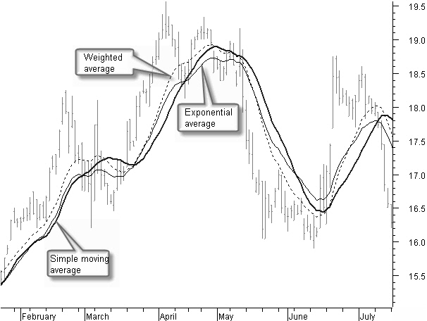
Figure 4.35: Simple, exponential and weighted moving average.

The thick, black curve in the chart of figure 4.35 is a 20-day simple moving average.

Exponential Moving Average

An exponential moving average gives more weight, percentage wise, to the individual prices in a range, based on the following formula:

EMA = (price * EMA %) + (previous EMA * (1 – EMA %))

Most investors do not feel comfortable with an expression related to percentage in the exponential moving average; rather, they feel better using a time period.
If you want know the percentage in which to work using a period, the next formula gives you the conversion:

A time period of three days corresponds to an exponential percentage of:

The thin, black curve in figure 4.35 is a 20-day exponential moving average.

Weighted Moving Average

A weighted moving average puts more weight on recent data and less weight on older data.

A weighted moving average is calculated by multiplying each data with a factor from day “1” till day “n” for the oldest to the most recent data; the result is divided by the total of all multiplying factors.

In a 10-day weighted moving average, there is 10 times more weight for the price today in proportion to the price 10 days ago. Likewise, the price of yesterday gets nine times more weight, and so on.

The thin, black dashed curve in figure 4.35 is a 20-day weighted moving average.

 

Simple, Exponential, or Weighted?

If we compare these three basic averages, we see that the simple average has the most smoothing, but generally also the biggest lag after price reversals.

The exponential average lies closer to the price and also will react faster to price swings. But shorter period corrections also are visible in this average because of a less smoothing effect.

Finally, the weighted average follows the price movement even more closely.

Determining which of these averages to use depends on your objective.  If you want a trend indicator with better smoothing and only little reaction for shorter movements, the simple average is best.

If you want a smoothing where you can still see the short period swings, then either the exponential or weighted moving average is the better choice.

Technical Analysis Averages 

Importance of the 20-, 50-, and 200-day Simple Averages

You must pay special attention to support and resistance of the 20-, 50-, and 200-day simple moving average. Additionally, the 20-day simple moving average is a nice tool to help you estimating the inclination of the shorter term trendline.

  

The 20-, 50-, and 200-day simple moving averages were mostly used in the past before the advent of personal computers. A simple average was used because the calculation was simple; longer periods were used because the movements in those days took time to take off and to complete.

This tradition is still alive today in the sense that investors still watch these averages. That is the reason why prices generally experience support and resistance at the level of these averages.

Figure 4.36: The 20, 50 and 200 days moving average.

In figure 4.36, note how the 20-day average gives direction to the shorter period price move and often runs parallel with a trendline.

The 50-day moving average gives direction to the medium-time period. If the price is moving above this average, it is good to have this share in your portfolio. If the price, however, moves below the 50-day average, it is better not to have this share in possession.

The 200-day moving average is important for a look at the long-term trend.

Around the 50- and the 200-day averages, you will almost always notice some form of support or resistance.

Technical Analysis Averages 

TEMA Average

The TEMA average is generally not used directly on a chart. This average is however used in many formulas to smooth longer periods of data with only a small amount of lag.

The TEMA, or Triple Exponential Moving Average, was introduced by Patrick Mulloy in Technical Analysis of Stocks & Commodities magazine, February 1994

  

TEMA is not simply a triple exponential moving average, as you probably would assume from the name. The intention of TEMA is to limit the typical lag of an average.
An ‘n’ day exponential average (EMA) has a smoothing factor alpha of:  

  

and a delay of 

.

The larger the average period n, the better the smoothing, but, unfortunately, the larger the delay. TEMA uses a technique of John Wilder Tukey to compensate the delay. The data is sent several times through the same filter and combined afterward:

TEMA = (3*EMA – 3*EMA(EMA)) + EMA(EMA(EMA))

The application of the TEMA average makes most sense if we want to smooth larger data periods, whereas the delay must remain as small as possible.

Figure 4.37: TEMA average.

Compare in figure 4.37 the 50-day TEMA average with the 20-day exponential average. You can see that the much longer TEMA average is at least as fast at the reversal points as the exponential average.

Technical Analysis Averages 

TEMA Average

The TEMA average is generally not used directly on a chart. This average is however used in many formulas to smooth longer periods of data with only a small amount of lag.

The TEMA, or Triple Exponential Moving Average, was introduced by Patrick Mulloy in Technical Analysis of Stocks & Commodities magazine, February 1994.

  

TEMA is not simply a triple exponential moving average, as you probably would assume from the name. The intention of TEMA is to limit the typical lag of an average.
An ‘n’ day exponential average (EMA) has a smoothing factor alpha of:  

  

and a delay of 

.

The larger the average period n, the better the smoothing, but, unfortunately, the larger the delay. TEMA uses a technique of John Wilder Tukey to compensate the delay. The data is sent several times through the same filter and combined afterward:

TEMA = (3*EMA – 3*EMA(EMA)) + EMA(EMA(EMA))

The application of the TEMA average makes most sense if we want to smooth larger data periods, whereas the delay must remain as small as possible.

Figure 4.37: TEMA average.

Compare in figure 4.37 the 50-day TEMA average with the 20-day exponential average. You can see that the much longer TEMA average is at least as fast at the reversal points as the exponential average.

Technical Analysis Averages 

Limiting the Lag

Interesting is the use of a technique to limit as much as possible the lagging nature of an average. We make use of this technique in all kind of formulas and applications to have enough smoothing without the side effect of too much lag.

Principles for limiting the lag (zero-lagging) of an average were introduced by Dr. Joe Sharp inStocks & Commodities magazine, January 2000. 

An application in MetaStock® formula language for a zero-lagging simple moving average on the closing prices is as follows:

Period:= Input(‘Which period?’,1,250,10);
SMA1:= Mov(CLOSE,Period,S);
SMA2:= Mov(SMA1,Period,S);
Difference:= SMA1 - SMA2;
ZeroLagSMA:= SMA1 + Difference;
ZeroLagSMA

Figure 4.38: Averages zero-lagging application.

The zero-lagging principle in figure 4.38 clearly shows less lag compared to the standard simple moving average.

The reversals are faster, but the zero-lagging average more closely follows the price move, so there is less smoothing.